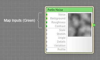
Map inputs, together with map components, are essential for building filters – they provide parameter mapping. Mapping means defining the value of a parameter separately for each area of the image. To map a parameter, you should connect a map component to the input corresponding to this parameter. A non-mapped parameter, say, a Contrast slider set to 55, has the same value of 55 across the entire image, while a mapped Contrast can have a different value for each area of the output image based on the brightness of the component connected to the map input.
How Mapping Works
For color inputs, such as Color 1, 2 and 3 in 3-Color Gradient, mapping is usually pretty obvious – instead of a 'flat' color defined by a color swatch in the component properties, the corresponding areas are filled with the image provided by the connected component:
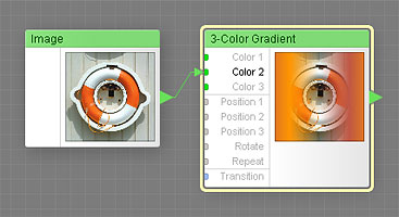
The supplied image replaces one of the gradient colors.
For non-color map inputs such as Contrast in Brightness / Contrast, mapping is a bit more complex – the value of the corresponding parameter is defined for various image areas separately by the brightness of the image supplied by the connected component.
In the example below, a black-to-white gradient is connected to the Contrast input of the Brightness / Contrast component. Since the Contrast slider has the range of -100 to 100, black areas of the gradient will correspond to the contrast of -100 (the left part of the thumbnail), white areas to the contrast of 100 (the right part of the thumbnail), and the gray levels in-between to intermediate contrast levels:
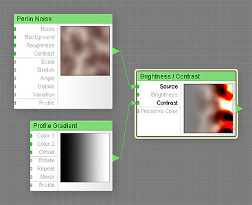
The brightness of the gradient defines the contrast level.
Another example: a gradient is connected to the Roughness input of the Perlin Noise component. Since the Roughness slider ranges from 0 to 100, black areas of the gradient will correspond to the roughness of 0, and white areas to the roughness of 100:
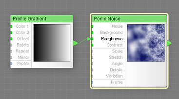
The brightness of the gradient defines the noise roughness.
If a full-color image is connected to a non-color map input, the color and alpha channel of the image are ignored, and only the brightness is used. Technically, values for the mapped non-color parameter are calculated as follows. The supplied image is converted into grayscale by averaging its R, G, and B channels, and this grayscale level is used to calculate the parameter value: white areas correspond to the maximum value, black areas to minimum value, and the values in-between are represented by intermediate grayscale levels.
Mapping and HDR Colors
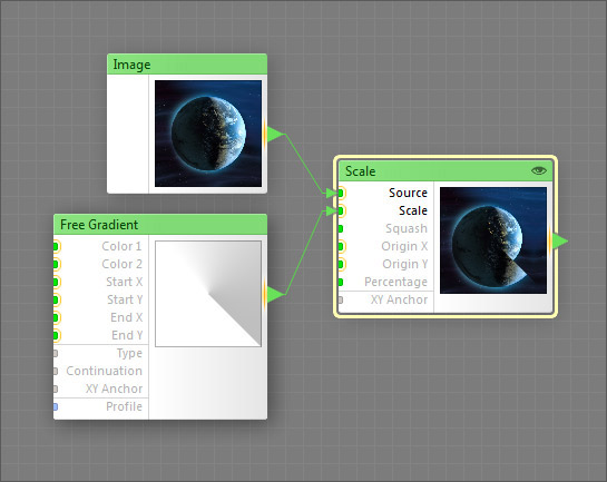
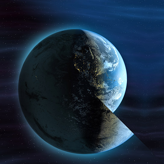
The real reason why we introduced unlimited HDR colors in Filter Forge is their ability to provide precise mapping of rangeless, unlimited parameters such as the scale factor in the Scale component or the coordinates of gradient endpoints in the Free Gradient component.
Values of HDR inputs, for example Origin X and Origin Y which define coordinates of origin points in the Rotate and Scale components, can range from tiny fractions to trillions, positive or negative. For example, you can have a rotation point placed five billion pixels to the right of the image's boundary. With unlimited HDR colors you can map these parameters with components that output HDR colors. In the example below, we map the scale factor with an HDR angular gradient whose brightness is ranging from 0.7 to 2:
Using negative HDR colors for parameter mapping is especially useful for controlling point coordinates. Take, for example, the Free Gradient component. It lets you specify the X and Y coordinates of both gradient endpoints. If Filter Forge had only positive finite colors, it would be impossible to place the endpoint beyond the image boundaries via parameter mapping.
With HDR colors, you can map the endpoint coordinates with a component that outputs negative HDR colors, allowing you to vary the point position in any way you want. You can do the same with rotation axis of the Rotate component, or with the scaling origin point of the Scale component, or the corners of the Free Rectangle, or the centers of Free Ellipse and Free Polygon.
Mapping and Curve Components
Most curve components also have map inputs. Connecting a map component to a map input of a curve component causes the curve to have a different shape for different areas of the image. Let's consider two examples below. In the first example, the Width input of the Impulse component has a constant value across the entire image, which produces a gradient stripe of a constant width:
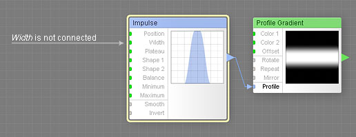
Width is not connected, its value is constant.
In the second example, Width is mapped with a left-to-right Profile Gradient. This results in the impulse width of 0 on the left side of the thumbnail, and the impulse width of 100 on the right side of the thumbnail. As a result, the gradient stripe has zero width on the left and 100% width on the right:
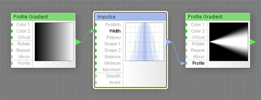
Width is mapped with a gradient.
Note that the curve thumbnail above shows multiple 'layers' of the curve, allowing you to get the idea of what shapes the mapped curve can assume across the image.